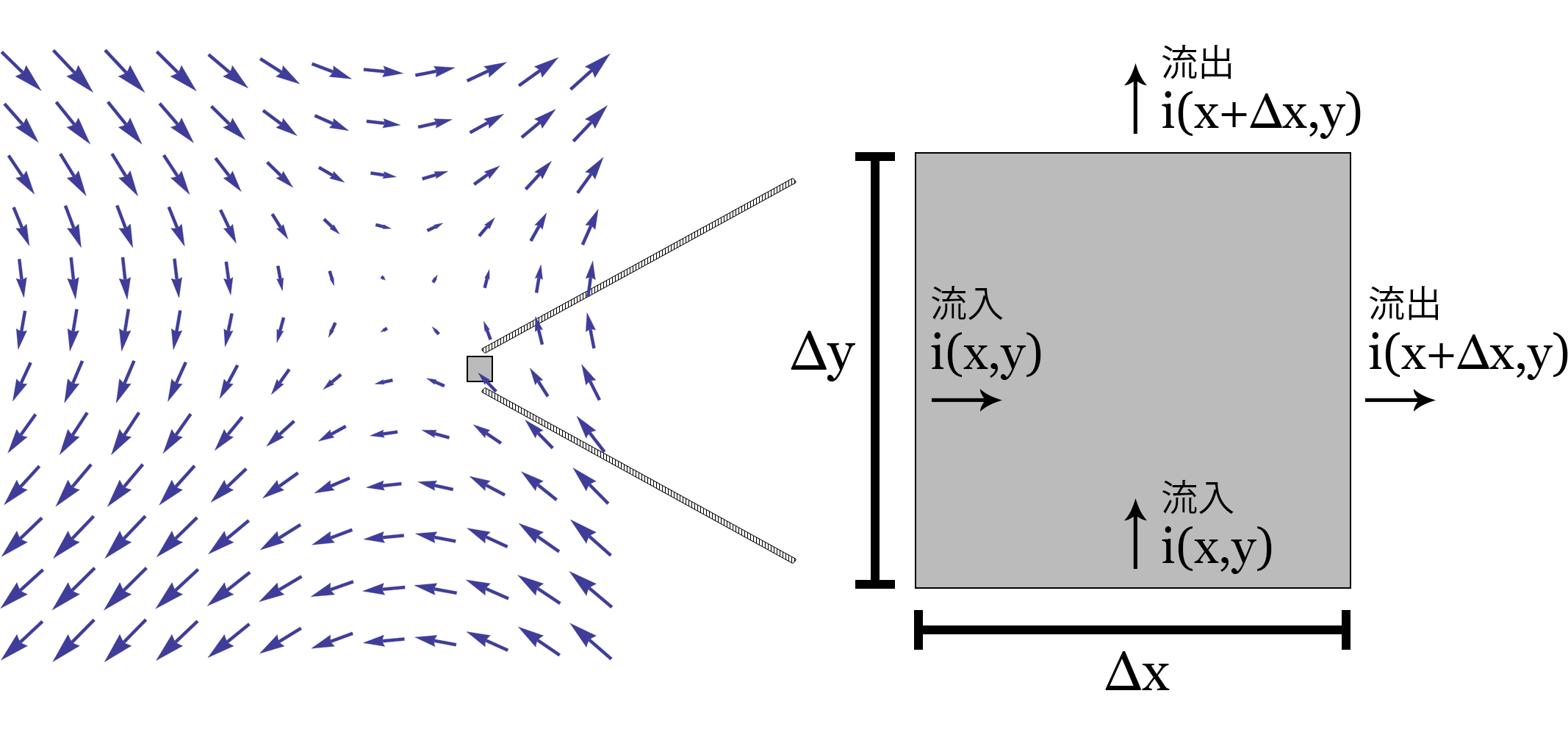
Figure 4.1: Extracting cells in the differential interval (Δx, Δy) from the vector field
In this chapter, we will explain the fluid simulation by the lattice method using Compute Shader.
https://github.com/IndieVisualLab/UnityGraphicsProgramming/
It is stored in Assets / StabeFluids of.
In this chapter, we will explain the fluid simulation by the lattice method and the calculation method and understanding of mathematical formulas necessary for realizing them. First of all, what is the grid method? In order to explore its meaning, let's take a closer look at how to analyze "flow" in fluid mechanics.
Fluid mechanics is characterized by formulating a natural phenomenon, "flow," and making it computable. How can this "flow" be quantified and analyzed?
If you go straight to it, you can quantify it by deriving the "flow velocity when the time advances for a moment". To put it a little mathematically, it can be rephrased as an analysis of the amount of change in the flow velocity vector when differentiating with time.
However, there are two possible methods for analyzing this flow.
One is to measure the flow velocity vector of each fixed lattice space by dividing the hot water in the bath into a grid when imagining the hot water in the bath.
And the other is to float a duck in the bath and analyze the movement of the duck itself. Of these two methods, the former is called the "Euler's method" and the latter is called the "Lagrange's method".
Now, let's get back to computer graphics. There are several simulation methods for fluid simulation, such as "Euler's method" and "Lagrange's method", but they can be roughly divided into the following three types.
As you can imagine from the meaning of Chinese characters, the grid method creates a grid-like "field" when simulating the flow, like the "Euler's method", and when it is differentiated with time, it is It is a method of simulating the speed of each grid. In addition, the particle method is a method of simulating the advection of the particles themselves, focusing on the particles, such as the "Lagrange method".
Along with the lattice method and particle method, there are areas of strength and weakness in each other.
The lattice method is good at calculating pressure, viscosity, diffusion, etc. in fluid simulation, but not good at advection calculation.
On the contrary, the particle method is good at calculating advection. (You can imagine
these strengths and weaknesses when you think of how to analyze Euler's method and Lagrange's method.) To supplement these, the lattice method + particle method represented by the FLIP method. There are also methods that complement each other's areas of expertise.
In this paper, we will explain the implementation method of fluid simulation and the necessary mathematical formulas in the simulation based on Stable Fluids, which is a paper on incompressible viscous fluid simulation in the lattice method by Jon Stam published at SIGGRAPH 1999. ..
First, let's look at the Navier-Stokes equation in the grid method.
\dfrac {\partial \overrightarrow {u}} {\partial t}=-\left( \overrightarrow {u} \cdot \nabla \right) \overrightarrow {u} + \nu \nabla ^{2} \overrightarrow {u} + \overrightarrow{f}
\dfrac {\partial \rho} {\partial t}=-\left( \overrightarrow {u} \cdot \nabla \right) \rho + \kappa \nabla ^{2} \rho + S
\nabla \cdot \overrightarrow{u} = 0
Of the above, the first equation represents the velocity field and the second represents the density field. The third is the "continuity equation (conservation of mass)". Let's unravel these three formulas one by one.
First, let's unravel the "continuity equation (conservation of mass)", which is short as an equation and works as a condition when simulating an "incompressible" fluid.
When simulating a fluid, it is necessary to make a clear distinction between compressible and incompressible objects. For example, if the target is a gas whose density changes with pressure, it will be a compressible fluid. Conversely, objects with a constant density, such as water, are incompressible fluids.
Since this chapter deals with incompressible fluid simulations, the divergence of each cell in the velocity field should be kept at zero. That is, it offsets the inflow and outflow of the velocity field and keeps it at zero. If there is an inflow, it will flow out, so the flow velocity will propagate. This condition can be expressed by the following equation as a continuity equation (conservation of mass).
\nabla \cdot \overrightarrow{u} = 0
The above means that "divergence is 0". First, let's check the formula of "divergence".
\nabla \cdot \overrightarrow{u} = \nabla \cdot (u, v) = \dfrac{\partial u}{\partial x} + \dfrac{\partial v}{\partial y}
\ nabla (nabla operator) is called the vector differential operator. For example, assuming that the vector field is two-dimensional, the partial differential of \ left (\ dfrac {\ partial} {\ partial x} _, \ dfrac {\ partial} {\ partial y} \ right) is calculated as shown in the figure. It acts as an operator that simplifies the notation of partial differential when taking. Since the \ nabla operator is an operator, it has no meaning by itself, but the operation content changes depending on whether the expression to be combined together is an inner product, an outer product, or just a function such as \ nabla f .
This time, let's explain "divergence" which takes the inner product of partial differential. First, let's see why this formula means "divergence".
In order to understand the divergence, let's first cut out one cell in the lattice space as shown below.
Figure 4.1: Extracting cells in the differential interval (Δx, Δy) from the vector field
Divergence is the calculation of how many vectors flow out and flow into one cell of a vector field. The outflow is + and the inflow is-.
As mentioned above, the divergence is the amount of change between the specific point x in the x direction and the slightly advanced \ Delta x when looking at the partial differential when the cell of the vector field is cut out, and the specific amount in the y direction. It can be calculated by the inner product of the amount of change between the point y and the slightly advanced \ Delta y . The reason why the outflow can be obtained by the inner product with the partial differential can be proved by performing a differential operation on the above figure.
\ frac {i (x + \ Delta x, y) \ Delta y - i (x, y) \ Delta y + j (x, y + \ Delta y) \ Delta x - j (x, y) \ Delta x } {\ Delta x \ Delta y}
= \ frac {i (x + \ Delta x, y) - i (x, y)} {\ Delta x} + \ frac {j (x, y + \ Delta y) - j (x, y)} { \ Delta Y}
Taking the limit from the above formula,
\ lim _ {\ Delta x \ to 0} \ frac {i (x + \ Delta x, y) - i (x, y)} {\ Delta x} + \ lim _ {\ Delta y \ to 0} \ frac {j (x, y + \ Delta y) - j (x, y)} {\ Delta y} = \ dfrac {\ partial i} {\ partial x} + \ dfrac {\ partial j} {\ partial y }
By doing so, we can see that the final equation is the equation of the inner product with the partial derivative.
Next, I will explain the velocity field, which is the main body of the lattice method. Before that, in implementing the Navier-Stokes equation of the velocity field, let's confirm the gradient and the Laplacian in addition to the divergence confirmed earlier.
\nabla f(x, y) = \left( \dfrac{\partial f}{\partial x}_,\dfrac{\partial f}{\partial y}\right)
\ nabla f (grad \ f) is the formula for finding the gradient. The meaning is which vector is finally directed by sampling the coordinates slightly advanced in each partial differential direction with the function f and synthesizing the obtained values in each partial differential direction. I will. In other words, it is possible to calculate a vector that points in the direction of the larger value when partially differentiated.
\Delta f = \nabla^2 f = \nabla \cdot \nabla f = \frac{\partial^2 f}{\partial x^2} + \frac{\partial^2 f}{\partial y^2}
The Laplacian is represented by a symbol with the nabla turned upside down. (Same as delta, but read from the context and make sure you don't make a mistake.) Also write
\ nabla ^ 2 f or \ nabla \ cdot \ nabla f and it is calculated as the second derivative.
Also, if you think about it by disassembling it, you can take the form of finding the divergence by taking the gradient of the function.
In terms of meaning, in the vector field, the part concentrated in the gradient direction has a lot of inflow, so when the divergence is taken, the part with a low gradient has a lot of springing out, so when the divergence is taken, it becomes +. I can imagine that.
Laplacian operators include scalar Laplacian and vector Laplacian, and when acting on a vector field, gradient, divergence, and rotation (cross product of ∇ and vector) are used.
\nabla^2 \overrightarrow{u} = \nabla \nabla \cdot \overrightarrow{u} - \nabla \times \nabla \times \overrightarrow{u}
However, only in the case of the Cartesian coordinate system, the gradient and divergence can be obtained for each component of the vector and can be obtained by combining them.
\nabla^2 \overrightarrow{u} = \left(
\dfrac{\partial ^2 u_x}{\partial x^2}+\dfrac{\partial ^2 u_x}{\partial y^2}+\dfrac{\partial ^2 u_x}{\partial z^2}_,
\ dfrac {\ partial ^ 2 u_y} {\ partial x ^ 2} + \ dfrac {\ partial ^ 2 u_y} {\ partial y ^ 2} + \ dfrac {\ partial ^ 2 u_y} {\ partial z ^ 2} _,
\dfrac{\partial ^2 u_z}{\partial x^2}+\dfrac{\partial ^2 u_z}{\partial y^2}+\dfrac{\partial ^2 u_z}{\partial z^2}
\right)
This completes the confirmation of the mathematical formulas required to solve the Navier-Stokes equation in the grid method. From here, let's look at the velocity field equation for each term.
\dfrac {\partial \overrightarrow {u}} {\partial t}=-\left( \overrightarrow {u} \cdot \nabla \right) \overrightarrow {u} + \nu \nabla ^{2} \overrightarrow {u} + \overrightarrow {f}
Of the above, \ overrightarrow {u} is the flow velocity, \ nu is the kinematic viscosity, and \ overrightarrow {f} is the external force (force).
You can see that the left side is the flow velocity when the partial differential is taken with respect to time. On the right side, the first term is the advection term, the second term is the diffusion viscosity term, the third term is the pressure term, and the fourth term is the external force term.
Even if these can be done collectively at the time of calculation, it is necessary to implement them in steps at the time of implementation.
First of all, as a step, if you do not receive an external force, you cannot make a change under the initial conditions, so I would like to start with the external force term in the fourth term.
This is simply the part that adds the vectors from the outside. In other words, when the velocity field is 0 in the initial condition, the vector is added to the corresponding ID of RWTexture2D from the UI as the starting point of the vector or some event.
The kernel of the external force term of the compute shader is implemented as follows. Also, describe the definitions of each coefficient and buffer that will be used in the compute shader.
float visc; //Dynamic viscosity coefficient
float dt; // delta time
float velocityCoef; //external force coefficient of velocity field
float densityCoef; //Density outside pressure coefficient

// xy = velocity, z = density, fluid solver to pass to drawing shader
RWTexture2D<float4> solver;
//density field, density field
RWTexture2D<float>  density;
//velocity field, velocity field
RWTexture2D<float2> velocity;
// xy = for vel, z = for dens. when project, x = p, y = div
// Save the buffer one step before and the temporary buffer when saving the mass
RWTexture2D<float3> prev;
// xy = velocity source, z = density source External force input buffer
Texture2D source;

[numthreads(THREAD_X, THREAD_Y, THREAD_Z)]
void AddSourceVelocity(uint2 id : SV_DispatchThreadID)
{
    uint w, h;
    velocity.GetDimensions(w, h);

    if (id.x < w && id.y < h)
    {
        velocity[id] += source[id].xy * velocityCoef * dt;
        prev[id] = float3(source[id].xy * velocityCoef * dt, prev[id].z);
    }
}
The next step is to implement the second term, the diffusion viscosity term.
\nu \nabla ^{2} \overrightarrow {u}
When there are values on the left and right of the \ nabla operator and \ Delta operator, there is a rule that "acts only on the right element", so in this case, leave the kinematic viscosity coefficient once and leave the vector Laplacian part. Think first.
With vector Laplacian for the flow velocity \ overright arrow {u} , the gradient and divergence of each component of the vector are taken and combined, and the flow velocity is diffused adjacently. By multiplying it by the kinematic viscosity coefficient, the momentum of diffusion is adjusted.
Here, since the gradient of each component of the flow velocity is taken and diffused, inflow from the adjacency and outflow to the adjacency occur, and the phenomenon that the vector received in step 1 affects the adjacency can be understood. think.
In terms of mounting, some ingenuity is required. If implemented according to the formula, if the diffusivity obtained by multiplying the viscosity coefficient by the differential time / number of lattices becomes high, vibration will occur, convergence will not be achieved, and the simulation itself will eventually diverge.
Iterative methods such as the Gauss-Seidel method, Jacobi method, and SOR method are used here to make the diffusion stable. Here, let's simulate with the Gauss-Seidel method.
The Gauss-Seidel method is a method of converting a formula into a linear equation consisting of unknowns for its own cell, using the calculated value immediately at the next iteration, and chaining it to converge to an approximate answer. The higher the number of iterations, the more accurate the values will converge, but graphics in real-time rendering require better frame rates and aesthetics rather than accurate results, so iterations are machine. Adjust for performance and appearance.
#define GS_ITERATE 4

[numthreads(THREAD_X, THREAD_Y, THREAD_Z)]
void DiffuseVelocity(uint2 id : SV_DispatchThreadID)
{
    uint w, h;
    velocity.GetDimensions(w, h);

    if (id.x < w && id.y < h)
    {
        float a = dt * visc * w * h;

        [unroll]
        for (int k = 0; k < GS_ITERATE; k++) {
            velocity[id] = (prev[id].xy + a * (
                            velocity[int2(id.x - 1, id.y)] +
                            velocity[int2(id.x + 1, id.y)] +
                            velocity[int2(id.x, id.y - 1)] +
                            velocity[int2(id.x, id.y + 1)]
                            )) / (1 + 4 * a);
            SetBoundaryVelocity(id, w, h);
        }
    }
}
The SetBoundaryVelocity function above is a method for boundaries. Please refer to the repository for details.
\nabla \cdot \overrightarrow{u} = 0
Let's go back to the conservation of mass side before proceeding with the section. In the process so far, the force received in the external force term is diffused in the velocity field, but at present, the mass of each cell is not preserved, and the mass is in the place where it keeps springing out and the place where there is a lot of inflow. Is in an unsaved state.
As in the equation above, you must save the mass and bring the divergence of each cell to 0, so let's save the mass here.
In addition, when performing the mass conservation step with Compute Shader, the field must be fixed because the partial differential operation with the adjacent thread is performed. It was expected to speed up if the partial differential operation could be performed in the group shared memory, but when the partial differential was taken from another group thread, the value could not be obtained and the result was dirty, so here is a buffer. While confirming, proceed in 3 steps.
Divergence calculation from velocity field> Poisson's equation is calculated by Gauss-Seidel method> Subtract to velocity field, divide the
kernel into 3 steps of conservation of mass, and bring it to conservation of mass while determining the field. In addition, SetBound ~ system is a method call for the boundary.
//Quality preservation Step1.
// In step1, calculate the divergence from the velocity field
[numthreads(THREAD_X, THREAD_Y, THREAD_Z)]
void ProjectStep1(uint2 id : SV_DispatchThreadID)
{
    uint w, h;
    velocity.GetDimensions(w, h);

    if (id.x < w && id.y < h)
    {
        float2 uvd;
        uvd = float2(1.0 / w, 1.0 / h);

        prev[id] = float3(0.0,
                    -0.5 *
                    (uvd.x * (velocity[int2(id.x + 1, id.y)].x -
                              velocity[int2(id.x - 1, id.y)].x)) +
                    (uvd.y * (velocity[int2(id.x, id.y + 1)].y -
                              velocity[int2(id.x, id.y - 1)].y)),
                    prev [id] .z);

        SetBoundaryDivergence(id, w, h);
        SetBoundaryDivPositive(id, w, h);
    }
}

//Quality preservation Step2.
// In step2, the Poisson equation is solved by the Gauss-Seidel method from the divergence obtained in step1.
[numthreads(THREAD_X, THREAD_Y, THREAD_Z)]
void ProjectStep2(uint2 id : SV_DispatchThreadID)
{
    uint w, h;

    velocity.GetDimensions(w, h);

    if (id.x < w && id.y < h)
    {
        for (int k = 0; k < GS_ITERATE; k++)
        {
            prev[id] = float3(
                        (prev[id].y + prev[uint2(id.x - 1, id.y)].x +
                                      prev[uint2(id.x + 1, id.y)].x +
                                      prev[uint2(id.x, id.y - 1)].x +
                                      prev[uint2(id.x, id.y + 1)].x) / 4,
                        prev[id].yz);
            SetBoundaryDivPositive(id, w, h);
        }
    }
}

//Quality preservation Step3.
// In step3, set ∇ ・ u = 0.
[numthreads(THREAD_X, THREAD_Y, THREAD_Z)]
void ProjectStep3(uint2 id : SV_DispatchThreadID)
{
    uint w, h;

    velocity.GetDimensions(w, h);

    if (id.x < w && id.y < h)
    {
        float  velX, velY;
        float2 uvd;
        uvd = float2(1.0 / w, 1.0 / h);

        velX = velocity[id].x;
        velY = velocity[id].y;

        velX -= 0.5 * (prev[uint2(id.x + 1, id.y)].x -
                       prev[uint2(id.x - 1, id.y)].x) / uvd.x;
        velY -= 0.5 * (prev[uint2(id.x, id.y + 1)].x -
                       prev[uint2(id.x, id.y - 1)].x) / uvd.y;

        velocity[id] = float2(velX, velY);
        SetBoundaryVelocity(id, w, h);
    }
}
The velocity field is now in a state of conservation of mass. Since the inflow occurs at the place where the outflow occurs and the outflow occurs from the place where there is a lot of inflow, it is expressed like a fluid.
-\left( \overrightarrow {u} \cdot \nabla \right) \overrightarrow {u}
Lagrange's method is used for the advection term, but the work of back tracing the velocity field one step before and moving the value of the place where the velocity vector is subtracted from the corresponding cell to the current location Do this for each cell. When backtraced, it does not go back to the place where it fits exactly in the grid, so when advection, linear interpolation with the neighboring 4 cells is performed and the correct value is advected.
[numthreads(THREAD_X, THREAD_Y, THREAD_Z)]
void AdvectVelocity(uint2 id : SV_DispatchThreadID)
{
    uint w, h;
    density.GetDimensions (w, h);

    if (id.x < w && id.y < h)
    {
        int ddx0, ddx1, ddy0, ddy1;
        float x, y, s0, t0, s1, t1, dfdt;

        dfdt = dt * (w + h) * 0.5;

        // Back trace point index.
        x = (float)id.x - dfdt * prev[id].x;
        y = (float)id.y - dfdt * prev[id].y;
        // Clamp so that the points are within the simulation range.
        clamp(x, 0.5, w + 0.5);
        clamp(y, 0.5, h + 0.5);
        // Determining cells near the back trace point.
        ddx0 = floor(x);
        ddx1 = ddx0 + 1;
        ddy0 = floor(y);
        Dy1 = Dy0 + 1;
        // Save the difference for linear interpolation with neighboring cells.
        s1 = x - ddx0;
        s0 = 1.0 - s1;
        t1 = y - ddy0;
        t0 = 1.0 - t1;

        // Backtrace, take the value one step before by linear interpolation with the neighborhood, and substitute it for the current velocity field.
        velocity[id] = s0 * (t0 * prev[int2(ddx0, ddy0)].xy +
                             t1 * prev[int2(ddx0, ddy1)].xy) +
                       s1 * (t0 * prev[int2(ddx1, ddy0)].xy +
                             t1 * prev[int2(ddx1, ddy1)].xy);
        SetBoundaryVelocity(id, w, h);
    }
}
Next, let's look at the density field equation.
\dfrac {\partial \rho} {\partial t}=-\left( \overrightarrow {u} \cdot \nabla \right) \rho + \kappa \nabla ^{2} \rho + S
Of the above, \ overrightarrow {u} is the flow velocity, \ kappa is the diffusion coefficient, ρ is the density, and S is the external pressure.
The density field is not always necessary, but by placing the pixels on the screen diffused by the density field on each vector when the velocity field is calculated, it becomes possible to express a more fluid-like expression that flows while melting. I will.
As some of you may have noticed by looking at the formula of the density field, the flow is exactly the same as the velocity field, the difference is that the vector is a scalar and the kinematic viscosity coefficient \ nu is the diffusion coefficient. There are only three points, one that is \ kappa and the other that does not use the law of conservation of mass.
Since the density field is a field of change in density, it does not need to be incompressible and does not need to be conserved by mass. In addition, the kinematic viscosity coefficient and the diffusion coefficient have the same usage as coefficients.
Therefore, it is possible to implement the density field by making a kernel other than the mass conservation law of the kernel used in the velocity field earlier by lowering the dimension. I will not explain the density field on paper, but please refer to the density field as it is also implemented in the repository.
Fluids can be simulated by using the above velocity field, density field, and conservation of mass law, but let's take a look at the simulation steps at the end.
The above is the simulation step of StableFluid.
By executing and dragging on the screen with the mouse, it is possible to cause the following fluid simulation.
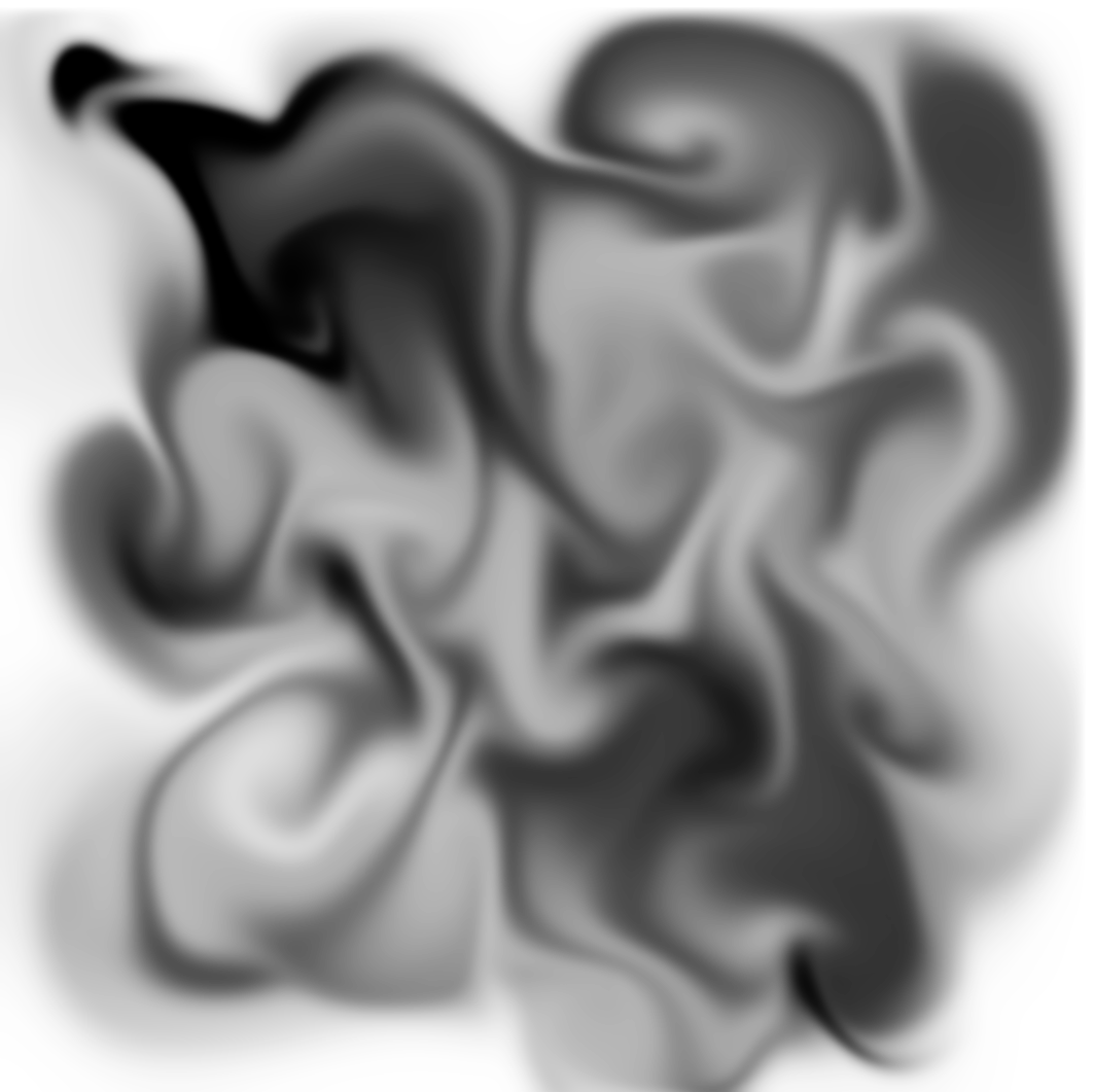
Figure 4.2: Execution example
Fluid simulation, unlike pre-rendering, is a heavy field for real-time game engines like Unity. However, due to the improvement of GPU computing power, it has become possible to produce FPS that can withstand even a certain resolution if it is two-dimensional. Also, if you try to implement the Gauss-Seidel iterative method, which is a heavy load for the GPU that came out on the way, with another process, or substitute the speed field itself with curl noise, etc. It will be possible to express fluids with lighter calculations.
If you have read this chapter and are interested in fluids even a little, please try "Fluid simulation by particle method" in the next chapter. Since you can approach the fluid from a different angle than the grid method, you can experience the depth of fluid simulation and the fun of mounting.